Machine Learning Workflow Review

Machine learning workflow defines all the necessary steps to train, test, and deploy a machine learning model. Machine learning workflow consists of data cleaning, feature engineering, algorithm selection, model training, validation of the model with test data and deploying the trained model in the production environment. In this article I will talk about all the steps of a machine learning workflow at an elevated level which will help you to prepare for future articles in this series.

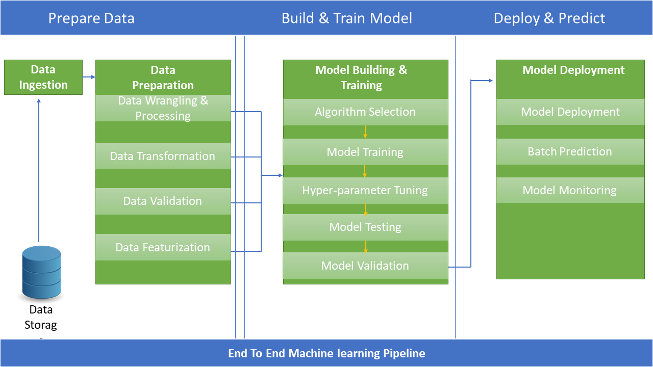
Figure 1 represents a typical end-to-end machine learning process where one can divide the entire pipeline in three key steps:

• Data preparation
• Build and train model
• Deploy and predict

Usually, the data preparation steps take the most amount of time. After that comes building and training models and the last step is deploying and monitoring models, which is the step to produnctionalize an AI model.

Data Preparation

Data preparation, which is the most important part of training a machine learning model, can have multiple steps:

• Training and testing data preparation
• Data cleaning, wrangling, and transformation
• Feature engineering

Training and Testing Data Preparation

A machine learning model is the result of a computer program that learned the pattern from an example data set and stored the patterns in a machine-readable format.

You provide a model with a data set to help it understand connections and patterns between the data. You can say that the model sees and learns from this example data.

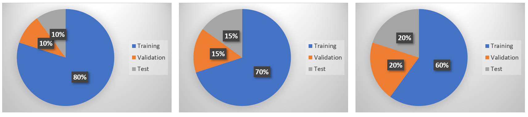
Data scientists usually divide their data sets in three different segments,

• Training set
• Validation set
• Testing set

Data that data scientists use to train a model is called a training set. After training is done, a validation set is used to validate performance. Later, a test data set is used to perform the realistic performance check on the algorithm. Using the test data set confirms if the model is accurate and can be used for predictive analytics or forecasting. The testing data set is data that the models have not seen during the training process. Testing data sets is particularly important as it helps us to understand the accuracy, reliability, and resilience of the model.

There is no fixed rule to determine the ratio of training, validation, and testing set. This depends on the data set size, problem type, and algorithm that data scientists have chosen. A rule of thumb that a lot of researchers follow is to have 70% data for training, 15% data for testing, and 15% data for validation.

If the number of hyper parameters to tune (trying out different structure of the model) is high based on the algorithm you choose, your ML model requires a larger validation set in that case.

Data Cleaning and Preprocessing

Building a machine learning model that understands the data requires a lot of data cleaning and pre-processing. Machines cannot learn the way humans learn from data, and for this reason the data needs to be prepared in a way that will be easier for models to consume. Data cleaning plays a significant role in building a good model. Common data cleaning steps that data scientists follow in the machine learning model development process are:

• Removing missing data / null values
• Removing duplicate data
• Identifying outliers' presence and removal from the data
• Handling erroneous data
• Identifying irrelevant data
• Clipping / handling outliers
• Removing similar values
• Removing Irrelevant data

Data Featurization

Data featurization defines the process of selecting a subset of relevant features, columns, or variables from a larger data set for constructing models. The main goal of feature selection is to improve the performance of a predictive model and reduce the computational cost of modeling by excluding redundant and irrelevant data.

Almost 70% of the success of the model depends on good feature selection / engineering process. Many data sets nowadays can have 100+ features for a data analyst to sort through! That is a ridiculous amount to process normally, which is where feature selection methods come in handy. They allow you to reduce the number of features included in a model without sacrificing predictive power.

Model quality depends on training data. If a validation set shows errors in training data, the model will be unusable. Proper validation techniques will help your machine learning workflow to avoid overfitting scenarios where a model has memorized a pattern of training data and performs badly on testing data.

Some of the common feature engineering techniques applied in day-to-day machine learning domains are:

• Imputation
• Discretization
• Categorical Encoding
• Feature Splitting
• Handling Outliers
• Variable Transformations
• Scaling
• Creating Features

Machine Learning Model Training

Supervised learning is an approach to creating artificial intelligence (AI), where a computer algorithm is trained on input data that has been labeled for a particular output.

The model is trained until it can detect the underlying patterns and relationships between the input data and the output labels, enabling it to yield accurate labeling results when presented with never-before-seen data.

Example of supervised learning,

• Loan screening
• Predicting insurance premiums
• Predicting survival chances
• Used car price prediction

The prediction task is a classification when the target variable is discrete. Example: predicting survival chances (0/1). There are distinct types of classification like binary classification, multi-class classification, multi-label classification, and imbalanced classification, etc.

The prediction task is a regression when the target variable is continuous. An example can be the prediction of the salary of a person given their education degree, previous work experience, geographical location, and level of seniority.

Unsupervised learning is an approach where no labels are given to the learning algorithm, leaving it on its own to find structure in its input. Unsupervised learning can be a goal in itself (discovering hidden patterns in data) or a means towards an end (feature learning). Example: clustering countries from GDP, import, export, life expectancy values.

Unsupervised learning is harder compared to supervised learning tasks.

Based on the problem type and the nature of the data set, we choose supervised learning or unsupervised learning during the development of the machine learning model.

Algorithm Selection

You choose the right algorithm based on the data set size, data set type, problem type, nature of the problem, available compute resources, etc. If you are solving a simple problem using a model where complex relations are not required and the data set is small, in that case you’ll likely use logistic regression or linear regression-based algorithms, but if we are dealing with larger data sets with complex relationships between variables, then you should use tree-based algorithms that are specialized for certain types of problem solving with more complexity.

Hyperparameter Tuning

Hyperparameters directly control model structure, function, and performance. Hyperparameter tuning allows data scientists to tweak model performance for optimal results. This process is an essential part of machine learning, and choosing appropriate hyperparameter values is crucial for success.

For example, assume you are using the learning rate of the model as a hyperparameter. If the value is too high, the model may converge too quickly with suboptimal results. Whereas if the rate is too low, training takes too long, and results may not converge. A good and balanced choice of hyperparameters results in accurate models and excellent model performance. Some examples are Bayesian optimization, grid search, random search, etc.

Model Validation

Once you train a model with the right algorithm, you need to validate the model to see if the model is giving the right predictions or not. There are different methodologies to validate a machine learning model; a few of the most common ones are described here:

Accuracy

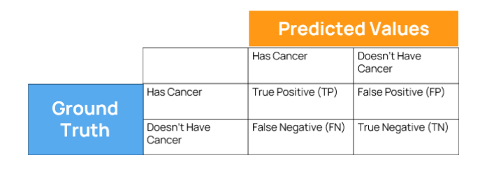
Classification accuracy is the simplest metric to use and implement and is defined as the number of correct predictions divided by the total number of predictions, multiplied by 100. Here, accuracy is Total (True Positive + True Negative) divided by all the possible cases (TP + TN + FP + FN) (Figure 3).

Confusion Matrix

A confusion matrix is a tabular visualization of the ground-truth labels versus model predictions. Each row of the confusion matrix represents the instances in a predicted class and each column represents the instances in an actual class. Figure 3 is the representation of a confusion matrix where you can see True Positive, True Negative, False Positive, and False Negative values based on predictions and ground truth of cancer use case. Here in Figure 3, we have the ground truth / true number of cancer results and the prediction values of machine learning model. We want to match ground truth values and predicted values to determine accuracy of the model, precision, recall and F1 score of the machine learning model.

Loss functions define what a good prediction is and is not. In short, choosing the right loss function dictates how well your overall learning is. Example: MAE (Mean Absolute Error), MSE (Mean Square Error), MSLE (Mean Squared Log Error).

Precision

Precision is the ratio of true positives and total positives predicted, P = TP / (TP + FP).

A precision score towards 1 will signify that your model did not miss any true positives and is able to classify well between correct and incorrect labeling of cancer patients (Figure 3).

Recall

A recall is the ratio of true positives to all the positives in ground truth (ground truth is represented by true occurrence / values and predicted values are from machine learning model). R = TP / (TP + FN)

Recall towards 1 will signify that your model did not miss any true positives and is able to classify well between correctly and incorrectly labeling of cancer patients of Figure 3.

A low recall score (<0.5) means your classifier has a high number of false negatives which can be an outcome of imbalanced class or untuned model hyperparameters.

F1 Score

The F1 score metric uses a combination of precision and recall. In fact, the F1 score is the harmonic mean of the two precision and recall which represents how balanced the overall model training is, F1 = 2 / (1/P + 1/R)

Coefficient of Determination

The coefficient of determination is a number between 0 and 1 that measures how well a statistical model predicts an outcome where 0 means does not predict the outcome; between 0 to 1 means partially predicts the outcome; 1 means the model perfectly predicts.

Model Deployment and Monitoring

The last part of the end-to-end machine learning pipeline is deployment of the machine learning model. Once you are comfortable with the model, you will deploy the model as an API endpoint so that you can make real time predictions or batch predictions using that model on real data. Machine learning operations play a crucial role here and once the model is deployed, we need to monitor the performance of the predictions to identify any data drift or model-related issues.

Conclusion

In this article I have looked at the general workflow of machine learning where I talked about end-to-end machine learning development process, data cleaning, processing, transformation, feature engineering steps, model selection, hyperparameter tuning and model evaluation. From our next articles, I will deep dive into MLOps steps of Azure machine learning and show details to use them.

This Stop: Machine Learning Workflow Review, article 4.

Series articles (will have links as they are published)

Article 1: MLOps Components and Machine Learning Platform Selection

Article 2: Azure Machine Learning Workspace Review

Article 3: Azure Machine Learning Compute Review

Article 4: Machine Learning Workflow Review (this article)

Article 5: Azure ML Notebook Selection and Development Process

Article 6: Connecting Data Sources with Azure ML Workspace

Article 7: Azure ML Security Review

Article 8: Azure ML Model Training

Article 9: Azure ML Model Registration and ML Job Automation

Article 10: Azure ML Model Deployment in ACI

Article 11: Azure ML Model Deployment in AKS

Article 12: Azure ML Model Health Monitoring

Article 13: Azure ML Model Drift and Data Drift Review

Article 14: Azure ML Model Retraining Pipeline

Article 15: Azure ML Model Result Analysis Dashboard with Power BI