Productivity Tip: Adding a Drop-Down List to Excel

Why would you want to add a drop-down list to an Excel spreadsheet, and not just create a form or a Power App? Well, you could do that if it better meets your needs — but sometimes you want something quick and easy within the app you’re working with, and then simply share out a link or, if it’s within one of the latest versions of Office, do some co-editing. Sometimes you may want to send out a spreadsheet for your users to fill out, or maybe you find yourself tracking repetitive data and want an easier way to collect information on your own.

Whatever the use case, this is a quick tip for generating drop-down lists to make that data entry just a little bit easier.

Creating a drop-down list

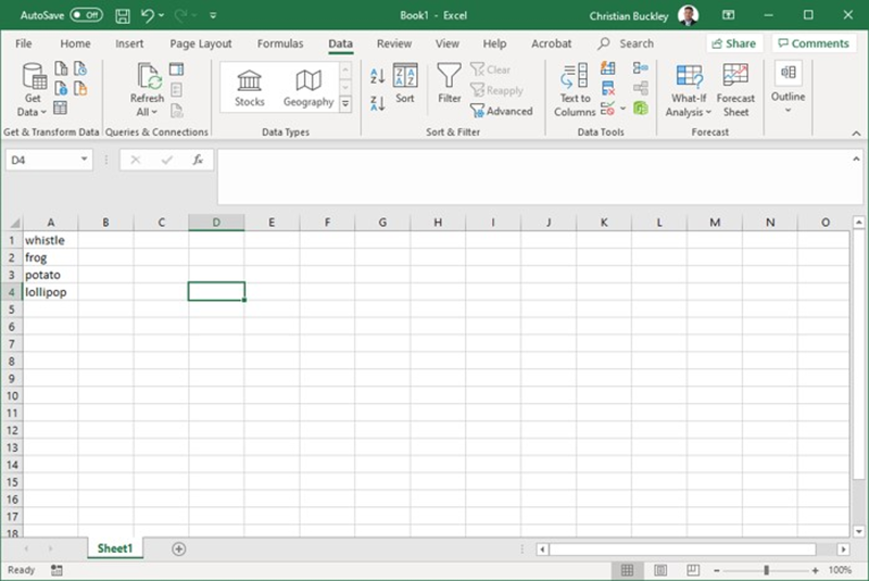
In Excel, the option to create a drop-down list is in the Data Validation feature. To get started, you’ll need to create a list. Create the list in cells A1:A4. Similarly, you can enter the items in a single row, such as A1:D1.

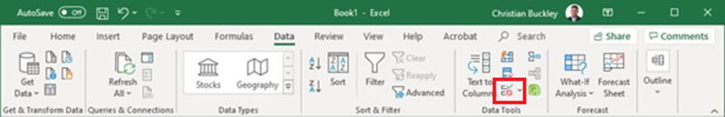
Next, you’ll want to select the position of your drop-down list. For this example, we’ll select cell E3. (You can position the drop-down list in almost any cell or even multiple cells.) Choose Data Validation from the Data menu.

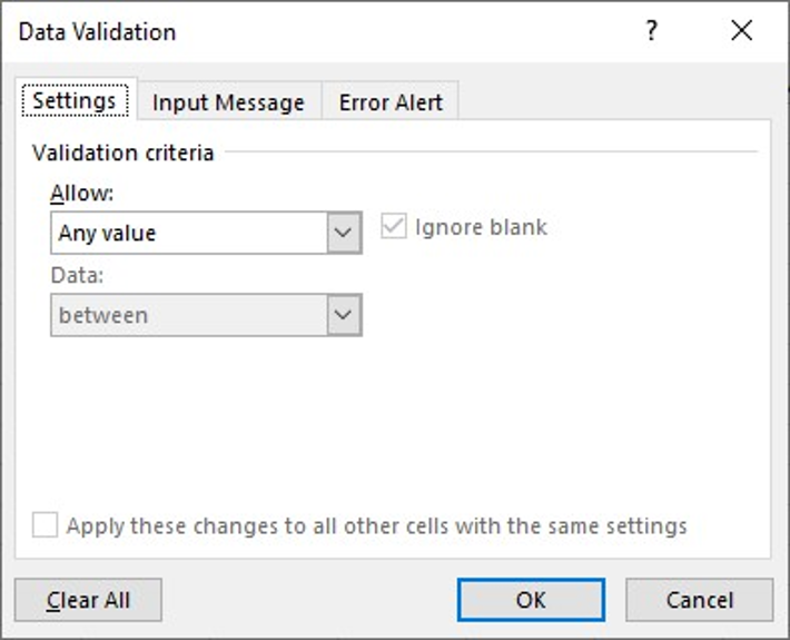
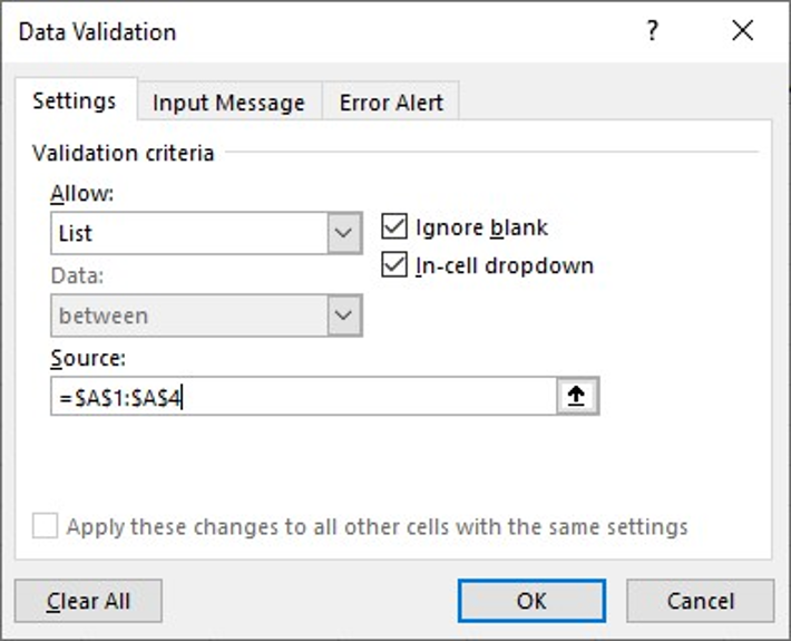
This opens the Data Validation dialog box.

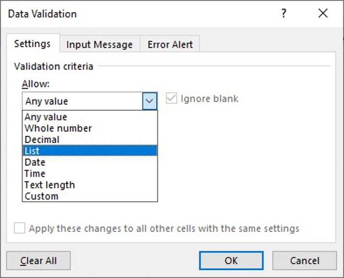
Choose List from the Allow option’s drop-down list. (See, they’re everywhere.)

Click the Source control to add your cursor, and then drag your mouse to highlight cells A1:A4. Alternately, you can also enter the reference (=$A$1:$A$4).

Make sure the In-cell dropdown option is checked. If you uncheck this option, Excel still forces users to enter only list values (A1:A4), but it won’t present a drop-down list. To finish the action, click OK.

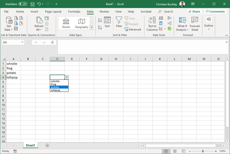
You can only see the drop-down…if you click on the cell.

Your users can now only select from one of the options in the drop-down list. If they try to enter their own data, they’ll receive an error message.

It’s a bit of manual effort to setup, but if you’re creating an Excel form that you want users to complete, this can save massive amounts of time and ensure that the data you capture is uniform and correct. You can copy-and-paste this drop-down cell to any other cells in your spreadsheet, and you can create as many different drop-downs like this as you’d like.

Hope you find this useful!